Lesson 2: NumPy Preliminaries

Instructor: Yuki Oyama, Prprnya

The Christian F. Weichman Department of Chemistry, Lastoria Royal College of Science

This material is licensed under CC BY-NC-SA 4.0

In this lesson, we will introduce some basic functionalities of the numpy library, which is a powerful library for numerical computing in Python. It provides support for arrays, matrices, and a wide range of mathematical functions. In this lesson, we will cover some of the basic features of NumPy.

Importing Libraries¶

In the first lesson, we introduced some basic concepts of variables and operations in Python, but in practice, we often need to use additional libraries to perform more complex tasks. Libraries are collections of pre-written code that provide additional functionality to Python. In this lesson, we will use the popular library: numpy.

To use a library, we need to import it first. We can do this using the import statement. For example, to import the numpy library, we can use the following code:

import numpy

After importing numpy, we can use its functions and methods to perform various operations on arrays and matrices. For example, we can check the value of $\pi$ (pi) using numpy:

pi

Oh, no... What’s going on? You should see a NameError after running the cell. This error indicates that pi is not defined. In fact, pi is a part of the numpy library, and we need to specify that we are using it from that library, which can be done by prefixing it with numpy.:

numpy.pi

However, typing numpy. every time can be tedious. To make it easier, we can import the library with an alias using the as keyword. This allows us to use a shorter name to refer to the library. For example, we can import numpy as np:

import numpy as np

You can even use nyanya as an alias if you want—

import numpy as nyanya
nyanya.pi

For the sake of our (and more possibly, other people’s!) mental health, let’s stick to np as the alias for numpy, which is the most commonly used alias in the scientific Python community. Now, you can check the value of π again:

import numpy as np
np.pi

Did you see the advantage of using aliases? It saves a lot of typing!

Common Math Functions¶

NumPy provides a wide range of mathematical functions:

For reference to more functions, see the NumPy documentation.

Let’s try this:

np.sqrt(2)

Also for this:

np.exp(1)

...and then:

np.cos(np.pi/2)

You will notice that the last output is not exactly zero. This is due to the limitations of floating-point arithmetic in computers, which can lead to small numerical errors. In practice, we often consider values very close to zero (e.g., within a small tolerance) as effectively zero.

Arrays¶

NumPy provides a powerful data structure called an array, which is a collection of elements of the same type. Arrays can be one-dimensional (like a list), two-dimensional (like a matrix), or even multidimensional. Let’s see an example of creating a one-dimensional array:

arr = np.array([1, 2, 3, 4, 5])
arr

In the code above, we created a one-dimensional array called arr using the np.array() function. The elements of the array are enclosed in square brackets and separated by commas. We can check the type of the variable arr using the type() function:

type(arr)

The output shows that arr is of type numpy.ndarray, which stands for “n-dimensional array”. This is rather a different type than the first lesson (int, float, etc.), but we don’t need to care the details.

We can also check the size of the array using the size attribute of the array, in which you need to add .size after the array name:

arr.size

Since arrays can only contain elements of the same type, if we try to create an array with mixed types, NumPy will automatically convert all elements to a common type. For example:

arr_mixed = np.array([1, 2.5, 3, 4.0, 5])
arr_mixed

Basic Operations¶

We can do some basic operations between arrays and numbers, such as addition, subtraction, multiplication, and division. For example:

arr + 1

We can also perform element-wise operations between two arrays of the same size. For example:

arr1 = np.array([10, 20, 30, 40, 50])
arr2 = np.array([1, 2, 3, 4, 5])
arr1 + arr2

We can also use some common mathematical functions on arrays. For example:

arr3 = np.array([0, np.pi/2, np.pi])
np.sin(arr3)

Indexing and Slicing¶

Sometimes we want to pick a single element from an array. We can do this using indexing. In Python, indexing starts from 0. Indices must be integers. For example, to access the first element of arr, we can use:

arr[0]

See what’s going on for this arr[-1]? The index -1 refers to the last element of the array. Similarly, -2 refers to the second-to-last element, and so on.

What if we try to access an index out of range?

arr[5]

Like the case that we want to access pi without importing numpy, we again see an error here, but this is a different type of error, an IndexError, which indicates that the index is out of range. In this case, the valid indices for arr are 0 to 4 (or -1 to -5), so trying to access index 5 results in an error. We will discuss error handling later.

If we want to access multiple elements from an array, we can use slicing. Slicing allows us to extract a portion of the array by specifying a range of indices. The syntax for slicing is array[start:stop], where start is the index of the first element to include, and stop is the index of the first element to exclude. Since start and stop are indices, they must be integers. For example:

arr[1:4]

If we set start equal to stop, we get an empty array:

arr[3:3]

Obviously, if start is greater than stop, we also get an empty array:

arr[4:2]

If we omit the start index, it defaults to 0. If we omit the stop index, it defaults to the length of the array. For example:

arr[:3]

Definitely, if we omit both start and stop, we get the entire array:

arr[:]

In addition to start and stop, we can also specify a step value using the syntax array[start:stop:step]. The step value determines the interval between elements to include in the slice. To avoid confusion, step must be a non-zero integer. If step is omitted, it defaults to 1. For example:

arrlong = np.array([1, 2, 3, 4, 5, 6, 7, 8, 9, 10])
arrlong[2:7:2]

For negative step, the slice is taken in reverse order. For example:

arrlong[::-1]

If we use a negative step, we need to ensure that the start index is greater than the stop index; otherwise, we will get an empty array. For example:

arrlong[7:2:-2]

Exercise : The code below generates an array of integers from 1 to 20.

arr_ex = np.arange(1, 21)

Write code to implement the following tasks:

• Extract the elements at odd indices (i.e., indices 1, 3, 5, ...) from this array using slicing.

• Subtract 1 from each of these extracted elements.

• Multiply each of the resulting elements by $\pi/6$.

• Calculate the cosine of each of these modified elements using np.cos().

Print the results of each step to verify your work.

2D Arrays¶

NumPy also supports multidimensional arrays. A two-dimensional array can be thought of as a matrix, with rows and columns. We can create a two-dimensional array using the np.array() function, by passing a list of lists. For example:

matrix = np.array([[1, 2, 3], [4, 5, 6], [7, 8, 9]])
matrix

Like one-dimensional arrays, we can check the type of the two-dimensional array:

type(matrix)

We notice that the type is still numpy.ndarray, which means that NumPy does not differentiate between one-dimensional and multidimensional arrays in terms of type. We can also check the size of the two-dimensional array, which is the total number of elements in the array:

matrix.size

For 2D arrays, we can also check the shape of the array using the shape attribute. The shape gives the number of rows and columns in the array in the form (rows, columns):

matrix.shape

The same operations we discussed for one-dimensional arrays can also be applied to two-dimensional arrays. For example, we can perform element-wise addition, subtraction, multiplication, and division between two matrices of the same shape. We can also use mathematical functions on each element of the matrix.

matrix2 = np.array([[9, 8, 7], [6, 5, 4], [3, 2, 1]])
matrix + matrix2

Indexing and slicing also work similarly for two-dimensional arrays. We can access individual elements, rows, or columns using indexing and slicing. Use the following matrix as an example:

a = np.array([[ 0,  1,  2,  3,  4,  5],
              [10, 11, 12, 13, 14, 15],
              [20, 21, 22, 23, 24, 25],
              [30, 31, 32, 33, 34, 35],
              [40, 41, 42, 43, 44, 45],
              [50, 51, 52, 53, 54, 55]])
a

To access a single row, we can use a single index. For example, to access the second row (which is [10, 11, 12, 13, 14, 15]), we can use:

a[1]

To access a single element, we should use two indices: the first index for the row and the second index for the column. For example, to access the element in the second row and third column (which is 12), we can use:

a[1][2]

A shortcut of doing this picking is:

a[1, 2]

This only applies to NumPy arrays, not Python lists.

However, accessing a single column is a bit tricky (for Python lists). Luckily, NumPy provides a convenient way to do this using slicing. Expanding the usage of the indexing shortcut above, we can replace any of the indices by a slice (start:stop:step).

Let’s see some examples:

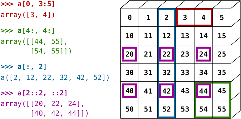
Image source: NumPy documentation

• The red one is a[0, 3:5], which picks the first row on the 4th to 5th columns (excluding the 6th column).

• The green one is a[4:, 4:], which picks the 5th to the last rows on the 5th to the last columns.

• The blue one is a[:, 2], which picks all the rows on the 2nd column.

• The purple one is a[2::2, ::2], which picks the 3rd to the last rows with a step of 2 on all the columns with a step of 2.

To verify these, you can run the following codes:

print(a[0, 3:5])    # Red
print(a[4:, 4:])    # Green
print(a[:, 2])      # Blue
print(a[2::2, ::2]) # Purple

Exercise : Using matrix slicing, extract the submatrix from the matrix a that includes the elements from the 2nd to the 4th rows and the 3rd to the 5th columns (inclusive of the start index and exclusive of the stop index, basically, a 3*3 submatrix centered around the element 23). Print the resulting submatrix.

Two Useful Functions for Arrays¶

Here are two useful functions to create arrays with evenly spaced values:

• np.arange(start, stop, step): Creates an array with evenly spaced values within a specified range.

• np.linspace(start, stop, num): Creates an array with a specified number of evenly spaced values between two endpoints.

For example, to create an array of integers from 0 to 9, we can use np.arange():

np.arange(0, 10, 1)

To create an array of odd numbers from 5 to 15, we can use:

np.arange(5, 16, 2)

For making an array from 0 to 1 with 5 evenly spaced values, we can use np.linspace():

np.linspace(0, 1, 5)

Finally, let’s create an array of 4 evenly spaced values from 0 to $\pi$:

np.linspace(0, np.pi, 4)

End-of-Lesson Problems¶

Problem 1: Play with Arrays¶

Using only methods introduced in this lesson:

1. Create a 1D array radians of 9 evenly spaced values from 0 to $\pi$ (inclusive) using np.linspace.

2. Compute two arrays:

   • s = np.sin(radians)

   • c = np.cos(radians)

3. Calculate t = s*s + c*c. Using slicing, extract all elements of t of odd index.

4. Using the existing 2D array matrix (already defined in the notebook), do the following:

   • Report matrix.size and matrix.shape.

   • Extract the last column using slicing/indexing.

   • Extract the submatrix consisting of all rows and the first two columns.

Problem 2: Quantum Harmonic Oscillator¶

Consider a one-dimensional quantum harmonic oscillator, but with a twist: the potential energy is added with a Dirac delta function at the origin. The potential is given by:

where $m$ is the mass of the particle, $\omega$ is the angular frequency, and $\alpha$ is a constant representing the strength of the delta potential. For simplicity, we set $m = 1$, $\omega = 1$, and $\alpha = 1$. That is,

The wavefunctions of the unperturbed harmonic oscillator are given by:

where $H_n$ are the Hermite polynomials. For simplicity, we set $\hbar = 1$. Substituting the values of $m$, $\omega$, and $\hbar$, we have:

Using NumPy, perform the following tasks:

1. Create a 1D array x of 200 evenly spaced values from -5 to 5 using np.linspace.

2. The code below defines a function harmonic_psi(n, x) that computes the wavefunction $\psi_n(x)$ for a given quantum number n and position array x. Test the value of $\psi_0$ at $x = 0$ and $x = 1$.

   from scipy.special import eval_hermite, factorial
   
   def harmonic_psi(n, x):
       return eval_hermite(n, x) * np.exp(-x ** 2 / 2) / np.sqrt(2 ** n * factorial(n)) / (np.pi) ** 0.25

3. Compute the values of $\psi_0$ from $x=-5$ to $x=5$ using the array x created before, and store the result in psi_0. Similarly, compute psi_1 to psi_5 for the first to fifth excited states. Create a 2D array psis where each row corresponds to a different quantum state (from $n=0$ to $n=5$) and each column corresponds to a position in x.

4. Now it’s time to bring our delta potential into play. The presence of the delta function at the origin modifies the wavefunctions, but it only affects the even states ($n=0, 2, 4, ...$). It’s a little bit more complicated to derive the even state solutions, but we can still keep our odd states. Create a new array psis_odd by slicing psis to keep only the odd states ($n=1, 3, 5$).

5. Run the code below, and you should be able to visualize the wavefunctions of the odd states. We will learn how to make plots like this later.

   from matplotlib import pyplot as plt
   
   plt.figure(figsize=(8, 6))
   
   for n in range(psis_odd.shape[0]):
       plt.plot(x, psis_odd[n], label=f'n={2*n+1}')
   
   plt.grid(linestyle='--')
   
   plt.legend()
   plt.show()

• NumPy Official Website

• Scientific Python Lectures

• Charles J. Weiss’s Scientific Computing for Chemists with Python

• An Introduction to Python for Chemistry

• GenAI for making paragraphs and codes(・ω< )★

• And so many resources on Reddit, StackExchange, etc.!