Lesson 2-extra 1: More about NumPy

Instructor: Yuki Oyama, Prprnya

The Christian F. Weichman Department of Chemistry, Lastoria Royal College of Science

This material is licensed under CC BY-NC-SA 4.0

After finishing Lesson 2, we have a basic understanding of NumPy, which still has many useful features worth learning. However, when processing large and complicated datasets, we need to use a more powerful tool, Pandas. In this lesson, we are going to learn the advanced features of NumPy in the first half, and Pandas in the second half.

Indexing and Masking¶

Our lesson begins by expanding the concept of indexing. NumPy arrays support not only integer indexing and slicing, but also several different but useful indexing methods. Let’s import NumPy first.

import numpy as np

Arbitrary Indexing¶

In lesson 2, we have learned how to get a single element from an array using integer indexing or get a regularly spaced subset of elements using slicing. However, NumPy also supports arbitrary indexing, which means that we can get elements using arbitrary conditions. Consider the following matrix:

mat = np.array([
    [1.1, 1.2, 1.3, 1.4, 1.5],
    [2.1, 2.2, 2.3, 2.4, 2.5],
    [3.1, 3.2, 3.3, 3.4, 3.5],
    [4.1, 4.2, 4.3, 4.4, 4.5],
    [5.1, 5.2, 5.3, 5.4, 5.5],
])
mat

We want to take some elements from the matrix, for example, the orange elements below:

These elements are located at the following indices: 3.1 at $(2, 0)$, 1.4 at $(0, 3)$, and 5.2 at $(4, 1)$. We can use two lists to represent the row indices and column indices of these elements, and use them to index the matrix:

rows = [2, 0, 4]
cols = [0, 3, 1]

mat[rows, cols]

Masking¶

Sometimes we want to filter out some elements from an array that meet certain conditions. Using the control flows we have learned in Lesson 1-extra, we can write a simple iteration combined with conditional statements to achieve this goal. However, NumPy provides a more convenient way to achieve this goal, which is called masking. For example, suppose we have some prime numbers such as

primes = np.array([2, 3, 5, 7, 11, 13, 17, 19, 23, 29, 31, 37])
primes

We want to find out all the primes $p$ of the form $4n + 3$ from the array. This condition can be expressed as p % 4 == 3 in Python. To create a mask that acts on primes using this condition, we just need to replace the p in the condition with primes:

mask = primes % 4 == 3
mask

The result is a boolean array that is True for all the elements that meet the condition and False for the rest (why?). We can use this mask to index the array to get the desired elements:

primes_filtered = primes[mask]
primes_filtered

Now check the mask again:

mask_filtered = primes_filtered % 4 == 3
mask_filtered

As you can see, all the elements in primes_filtered meet the condition. However, checking each element in the mask manually is not very efficient. To simplify this process, we can use the any() and all() methods of NumPy boolean arrays to check whether any or all the elements meet the condition:

mask.any(), mask.all(), mask_filtered.any(), mask_filtered.all()

The results of these two methods are np.True_ and np.False_, which are wrapped by NumPy from the built-in True and False in Python, so you can treat them as the same. For boolean array, the any() method returns True if at least one of the elements in the array is True, and the all() method returns True if all the elements in the array True.

Exercise : Imagine that we mark the grid points (points with integer coordinates) on the 2D plane and then draw a circle centered at the origin with a radius of $r$ (for simplicity, $r$ only takes integer values). Use masking to show how many grid points are in the circle (including the boundary). We can use the meshgrid() function to generate a grid of points, for example:

xrange = np.arange(2)
yrange = np.arange(3)
x, y = np.meshgrid(xrange, yrange)
x, y

Each pair of elements with the same index in x and y represents a grid coordinate.

Hint: the mask is also an array, which can be indexed using the mask itself.

Array Manipulation¶

The array in NumPy is very flexible, which has a series of methods that allow us to perform various operations on it.

Reshape¶

NumPy provides a convenient way to reshape arrays. Let’s create an 1D array first.

arr1d = np.arange(12)
arr1d

Check the size and shape of arr1d.

arr1d.size, arr1d.shape

The reshape() method of ndarray is used to reshape the array. We can pass the desired shape as positional arguments to the method.

arr2d = arr1d.reshape(3, 4)
arr2d

Now check the size and shape of arr2d.

arr2d.size, arr2d.shape

Note that the size of the reshaped array has to be the same as the original array, other a ValueError will be raised. For example, the shape (3, 4) is acceptable since $3 \times 4 = 12$, which equals to the size of arr1d, but the shape (2, 5) is not acceptable since $2 \times 5 = 10 \ne 12$.

arr1d.reshape(2, 5)

Another example for 3D array:

arr3d = arr1d.reshape(2, 2, 3)
arr3d

Check the size and shape of arr3d.

arr3d.size, arr3d.shape

Flatten¶

The flatten() method of ndarray can convert a multidimensional array into a 1D array.

arr2d.flatten()

Another example for 3D array:

arr3d.flatten()

Transpose¶

The transpose() method of ndarray returns an array with axes transposed. For 1D array, the transpose is the same as the original array, since an 1D array can be considered as a vector.

arr1d.transpose()

For 2D array, the transpose is the standard matrix transpose.

arr2d.transpose()

Check the shape of the transposed array.

arr2d.transpose().shape

For an $n$-D array, we can pass the axis indices as positional arguments, where the order indicates how the axes are permuted.

arr3d.transpose(1, 2, 0)

Check the shape of the transposed array.

arr3d.transpose(1, 2, 0).shape

If axes are not provided, then the shape of the array is reversed.

arr3d.transpose()

Now check the shape of the transposed array again.

arr3d.transpose().shape

Exercise : Use only one line of code to reorder arr1d, where all elements in the form $3n$ are moved to the front of the array, then $3n+1$ and $3n+2$. Your result should be like [0, 3, 6, 9, 1, 4, 7, 10, 2, 5, 8, 11].

Vectorization¶

NumPy arrays naturally support batch operations, which is convenient for performing operations on arrays. For example, we can perform element-wise operations on arrays by combining arrays and operators directly:

squares = np.arange(5) ** 2
squares

Most of the NumPy functions also support batch operations on arrays by passing arrays as arguments. For example, we can use the sqrt() function to calculate the square roots of the elements in squares:

np.sqrt(squares)

However, when we need to combine arrays with Python native functions, we have to use regular loops and iterations, otherwise we will encounter an TypeError.

import math
math.sqrt(squares)

Fortunately, NumPy provides a feature called vectorization, which can be used to convert Python native functions into vectorized functions that support array operations using decorator syntax.

@np.vectorize
def vec_sqrt(n: int | float) -> float:
    return math.sqrt(n)

vec_sqrt(squares)

Note: The type annotation int | float is used to indicate that the type of argument n can be either int or float, where the | symbol is used to indicate the union of two types.

Exercise : Define a vectorized function vec_parity(n) that returns the parity of n, which means 1 if n is odd and -1 if n is even. Apply the vectorized function to squares to check your result.

Broadcasting¶

When we need to combine arrays with different shapes, we can use the broadcasting mechanism provided by NumPy, which can be used to convert arrays with different shapes into arrays with the same shape. Somewhat counterintuitively, the vectorization is essentially a form of broadcasting if we consider scalars as arrays with shape (1,). Using the example from NumPy’s documentation:

a = np.array([1, 2, 3])
b = 2
a * b

The following code gives the same result as the previous one:

a = np.array([1, 2, 3])
b = np.array([2, 2, 2])
a * b

Comparing the results of the two codes above, we find that the array b in second code is stretched from the scaler b in the first code into the same shape as a, which can be visually represented as shown in the figure below.

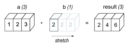
Image source: NumPy documentation

In general, two dimensions are compatible when they are equal or one of them is 1. When broadcasting, NumPy will attempt to treat one array as an element of the other array (in the sense of dimension compatibility). This means that the dimensions in the shape of the smaller array will be compatible with the dimensions in the trailing (i.e., rightmost) part of the shape of the larger array term by term. For example, the following code will broadcast the array b into the shape of a:

a = np.array([[ 0,  0,  0],
              [10, 10, 10],
              [20, 20, 20],
              [30, 30, 30]])
b = np.array([1, 2, 3])
a + b

Since b.shape == (3,), which is compatible to the trailing part of a.shape == (4, 3), the array b is possible to be broadcasted into the shape of a like the figure below:

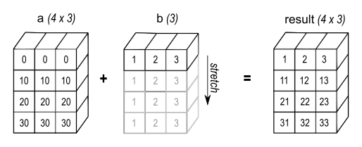
Image source: NumPy documentation

If the shapes of both a and b are not the trailing part of each other, then the arrays cannot be broadcasted. For example, the following code will raise a ValueError since a.shape == (4, 3) and b.shape == (4,), which are mismatch:

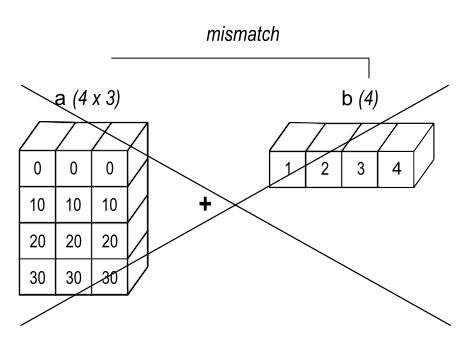
Image source: NumPy documentation

a = np.array([[ 0,  0,  0],
              [10, 10, 10],
              [20, 20, 20],
              [30, 30, 30]])
b = np.array([1, 2, 3, 4])
a + b

Finally, let’s introduce another way to force compatibility between two arrays:

a = np.array([0, 10, 20, 30])
b = np.array([1, 2, 3])
a[:, np.newaxis] + b

The np.newaxis is a special value that can be used to insert a new axis of dimension 1 into an array. In the example above, the array a is converted into the shape of (4, 1), which matches b.shape == (3,). The result is shown in the figure below:

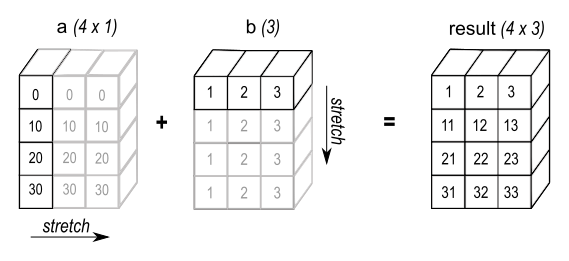
Image source: NumPy documentation

As a reference, here are some more examples of compatible shapes:

A      (2d array):  5 x 4
B      (1d array):      1
Result (2d array):  5 x 4

A      (2d array):  5 x 4
B      (1d array):      4
Result (2d array):  5 x 4

A      (3d array):  15 x 3 x 5
B      (3d array):  15 x 1 x 5
Result (3d array):  15 x 3 x 5

A      (3d array):  15 x 3 x 5
B      (2d array):       3 x 5
Result (3d array):  15 x 3 x 5

A      (3d array):  15 x 3 x 5
B      (2d array):       3 x 1
Result (3d array):  15 x 3 x 5

Here are examples of shapes that do not broadcast:

A      (1d array):  3
B      (1d array):  4 # trailing dimensions do not match

A      (2d array):      2 x 1
B      (3d array):  8 x 4 x 3 # second from last dimensions mismatched

Exercise : There are a three arrays in different shapes. Use the broadcasting rule to add them together to get a single array in the shape of a:

a = np.array([[ 0,   1,   2],
              [10, 100, 1000]])
b = np.array([1, 2, 3])
c = np.array([1, -1])

Linear Algebra in NumPy (numpy.linalg)¶

In computer science, linear algebra problems can often be transformed into array-based problems, making NumPy well-suited for solving such problems. The subpackage numpy.linalg provides a variety of linear algebra functions, including matrix multiplication, matrix inversion, eigenvalue decomposition, singular value decomposition, and so on.

Vectors and Matrices¶

Let’s first look at the basic linear algebra concepts: vectors and matrices. In NumPy, vectors and matrices can be modeled as ndarray objects. For example, the following code creates two arrays representing 3D vectors (mathematically, we denote them as $\mathbf{v}_1, \mathbf{v}_2 \in \mathbb{R}^3$):

v1 = np.array([1, 1, 4])
v2 = np.array([5, 1, 4])
v1, v2

The np.linalg.norm() function can be used to calculate the norm of a vector or matrix. We can use the ord parameter to specify the norm type. For example, the default value ord=2 indicates the Euclidean distance, ord=1 indicates the Manhattan distance, and ord=np.inf indicates the Chebyshev distance.

norm1 = np.linalg.norm(v1)
norm2 = np.linalg.norm(v2)

norm1, norm2

The np.dot() and np.cross() functions can be used to calculate the dot product and cross product of two vectors. For example:

np.dot(v1, v2), np.cross(v1, v2)

Now let’s look at the matrices. The function np.dot() can also be used to calculate the product of two matrices. Recall that the product of two matrices $A$ and $B$ can be represented as follows:

Image source: Wikipedia

The number of columns in $A$ must be equal to the number of rows in $B$, and thus we can take the dot product of each row in $A$ and each column in $B$ to obtain the product of $A$ and $B$. Now let’s define two matrices $M_1$ and $M_2$ and calculate their product:

M1 = np.array([
    [1, 0, 0],
    [0, 0, -1],
    [0, 1, 0],
])  # Rotating 90 degrees clockwise about the x-axis
M2 = np.array([
    [0, 1, 0],
    [1, 0, 0],
    [0, 0, 1],
])  # Reflecting about the plane y = x

np.dot(M1, M2)

Python 3.5 introduced the builtin @ operator as a dedicated infix operator for matrix multiplication, which is more concise and easier to read. Therefore, we can also write the above code as follows:

M = M1 @ M2
M

The @ operator can also be used to multiply a matrix and a vector. For example, let’s multiply the matrix $M$ with the standard basis vectors $\mathbf{e}_x, \mathbf{e}_y, \mathbf{e}_z \in \mathbb{R}^3$ to extract the columns of $M$:

ex, ey, ez = np.identity(3, dtype=int)
M @ ex, M @ ey, M @ ez

Note: The function np.identity() can be used to create an identity matrix in NumPy.

Furthermore, using the @ operator to multiply two vectors gives their dot product:

v1 @ v2

Exercise : Verify that $M$ is an orthogonal matrix by calculating $M^\top M$ and comparing the result with $I$, then calculate the dot product of $M\mathbf{v}_1$ and $M\mathbf{v}_2$, and compare it with the dot product of $\mathbf{v}_1$ and $\mathbf{v}_2$, which should be like:

Eigenvalues and Eigenvectors¶

In linear algebra, the eigenvalues and eigenvectors of a matrix are two fundamental properties of a matrix. By definition, if there exists some non-zero vector $\mathbf{x}$ such that $M\mathbf{x} = \lambda \mathbf{x}$, then $\lambda$ is an eigenvalue of $M$, and $\mathbf{x}$ is the corresponding eigenvector. For example, the matrix $\begin{bmatrix} 1 & 1 \\ 1 & -1 \end{bmatrix}$ has two eigenvalues $\lambda_1 = \sqrt{2}$ and $\lambda_2 = -\sqrt{2}$, and the corresponding eigenvectors are $e_1 = \begin{bmatrix} 1+\sqrt{2} \\ 1 \end{bmatrix}$ and $e_2 = \begin{bmatrix} 1-\sqrt{2} \\ 1 \end{bmatrix}$.

In Numpy, we can use the function np.linalg.eig() to calculate the eigenvalues and eigenvectors of a matrix, which will give results in complex numbers. Using $M$ as an example:

eigenvalues, eigenvectors = np.linalg.eig(M)
eigenvalues, eigenvectors

Note: The second return value eigenvectors can be considered as the matrix where each column is an eigenvector of $M$.

To verify the columns of eigenvectors are eigenvectors of $M$, we can evaluate the following equation for each eigenvalue $\lambda_i$ and corresponding eigenvector $\mathbf{x}_i$:

I = np.identity(3)
l1, l2, l3 = eigenvalues
e1, e2, e3 = eigenvectors.T  # Equivalent to eigenvectors.transpose()

((M - l1 * I) @ e1).round(), ((M - l2 * I) @ e2).round(), ((M - l3 * I) @ e3).round()

For hermitian matrices or real symmetric matrices, by the spectral theorem, the eigenvalues of a matrix are real, and the normalized eigenvectors form an orthonormal basis for the whole space. NumPy provides the np.linalg.eigh() and np.linalg.eigvalsh() functions to calculate the eigenvalues and eigenvectors of hermitian or real symmetric matrices, where the eigenvalues are sorted in ascending order. Using $M + M^\top$ as an example:

np.linalg.eigvalsh(M + M.T), np.linalg.eigh(M + M.T)

Exercise : Verify that the following two symmetric matrices has the same eigenvalues, and find the corresponding eigenvectors:

Trace and Determinant¶

In linear algebra, the trace of a matrix is the sum of the elements on the main diagonal of a square matrix, and the determinant of a square matrix is a scalar value that can be calculated using the parity of permutations. For example, the matrix

has trace

and determinant

We can use the np.trace() function to calculate the trace of a matrix, and use the np.linalg.det() function to calculate the determinant of a square matrix. Using $M$ as an example:

np.trace(M), np.linalg.det(M)

Inverse and Solving Linear Systems¶

In linear algebra, the inverse of a square matrix $A$ is another matrix $A^{-1}$ such that $AA^{-1} = A^{-1}A = I$. The determinant of an invertible matrix is always nonzero, otherwise the matrix is singular and cannot be inverted.

We can use the np.linalg.inv() function to calculate the inverse of a square matrix. Using $M$ as an example:

np.linalg.inv(M)

If we pass a non-invertible matrix to the function, it will raise LinAlgError("Singular matrix"):

np.linalg.inv(np.array([[1, 1], [-1, -1]]))

Exercise : We have already learned the least squares solution of a linear system $Ax = b$ in linear algebra. NumPy also provides the np.linalg.lstsq(A, b) function to solve linear systems. Now let’s solve the following linear system:

Note that np.linalg.lstsq() returns a tuple of four elements, where the first element is the least squares solution of the linear system. The remaining three elements will be explained in the End-of-Lesson Problems.

Decomposition or Factorization¶

In linear algebra, a matrix decomposition is a process of factorizing a matrix into a product of simpler matrices to get some useful information or solve some specific problems. NumPy provides several functions for matrix decomposition, which are listed here.

For example, the QR decomposition of a matrix $A$ says that $A = QR$, where $Q$ has orthonormal columns, and $R$ is an upper triangular matrix. We can use the np.linalg.qr() function to calculate the QR decomposition of a matrix:

np.linalg.qr(M)

Exercise : Do the QR decomposition of the following non-square matrices:

Check your linear algebra textbook to understand what the output means.

End-of-Lesson Problems¶

Problem 1: Hückel Method¶

In chemistry, Hückel method is an approximate method for calculating the energy levels of conjugated $\pi$-orbitals. It assumes that only adjacent $p$-orbitals interact with each other, and obtain the energy levels by solving the secular equation. Essentially, this is equivalent to solving the characteristic polynomial of a matrix, where the eigenvalues are the energy levels.

Using ethylene as an example, the $p$-orbitals contributed by the two carbon atoms are labeled $\phi_1$ and $\phi_2$ respectively, and the molecular orbitals $\psi_1$ and $\psi_2$ can be expressed as a linear combination of $\phi_1$ and $\phi_2$, which are

We record the energy level of a single $p$-orbital as $\alpha$, and the interaction energy between two adjacent $p$-orbitals as $\beta$. Then the energy levels $E_i$ of the molecular orbitals are the eigenvalues of the matrix in the following equation:

The characteristic polynomial is given by:

The roots of the characteristic polynomial give the energy levels:

Thus, we can solve the equations above to get the coefficients of the molecular orbitals:

Therefore, the molecular orbitals can be expressed as:

Giving $\alpha = -1087\ \text{kJ/mol}$ (the first ionization energy of a carbon atom) and $\beta = -252\ \text{kJ/mol}$ (derived from data in J. Chem. Educ. 1994, 71, 171), calculate $E_1$ and $E_2$ for ethylene, then compute the total $\pi$-electron energy of ethylene.

Note: Since the matrix is symmetric (why?), we can use np.linalg.eigvalsh() to calculate the eigenvalues of the matrix.

Now consider benzene, which has six $p$-orbitals labeled $\phi_1$ to $\phi_6$. Assume that benzene shares the same $\alpha$ and $\beta$ values as ethylene. Calculate the total $\pi$-electron energy of benzene using the same method.

The resonance energy of benzene is defined as the difference between the total $\pi$-electron energy of the benzene molecule and that of the hypothetical cyclohexatriene molecule, which can be approximated as three isolated ethylene molecules. Calculate the resonance energy of benzene, then compare it with the experimental value (by measuring the hydrogenation enthalpy of benzene) of approximately $152\ \text{kJ/mol}$. Consider whether the Hückel method gives a good approximation and why.

Problem 2: The Principle of Least Squares¶

We have already practiced how to use np.linalg.lstsq() to solve linear systems in the previous exercise. In this problem, we will try to solve the same linear system step by step using the principle of least squares. First, let’s review the linear system we want to solve:

A = np.array([
    [1, 1, 4],
    [5, 1, 4],
    [8, 1, 0],
    [8, 9, 3],
])
b = np.array([2, 2, 3, 3])

Then check the least square solution using np.linalg.lstsq().

Now let’s solve the linear system step by step. First, check whether the determinant of $A^\top A$ is zero.

If the determinant is nonzero, solve the linear system $A^\top A x = A^\top b$ directly, then compare the result with the least square solution obtained by np.linalg.lstsq().

The second value returned by np.linalg.lstsq() is the norm of the residual, which is the difference between $Ax$ and $b$. Now calculate the norm of the residual and compare it with the value returned by np.linalg.lstsq().

The third value returned by np.linalg.lstsq() is the rank of $A$. Use np.linalg.matrix_rank() to verify the rank of $A$.

The last value returned by np.linalg.lstsq() is the singular values of $A$, which are the square roots of the eigenvalues of $A^\top A$. Use np.linalg.svdvals() to calculate the singular values of $A$.

• NumPy Official Website

• GenAI for making paragraphs and codes(・ω< )★

• And so many resources on Reddit, StackExchange, etc.!